In the year 1834, a French scientist by the name Benoît Paul Émile Clapeyron discovered the Ideal Gas Equation, which finally put together the various behaviour of an ideal gas (a hypothetical gas whose molecules occupy negligible space, does not react with other substances, and obeys the gas laws perfectly) into one elegant equation

Where P is pressure Pascals, V is volume cubic meters, N is the number of molecules of gas, k is the Boltzmann constant at 1.3806488 × 10⁻²³, and T is temperature in Kelvin. However, this brainchild was not born completely out of a dash of pure genius. Instead, it was the product of decades of independent scientific inquiry on the topic of gas and its behaviour. Namely three separate previously discovered gas laws can be attributed to the synthesis of the Ideal Gas Equation. The first is Boyle’s law, which was discovered in 1662 by Irish scientist Robert Boyle, it states that under constant temperature, as the pressure of a gas increases, its volume decreases.

Where C is the proportionality constant NkT. The next law is what’s known as Charles’ Law which states that at constant pressure, as the temperature of a gas increases, so does its volume.

This time, the proportionality constant is Nk/P . Finally, the third law known as the Gay-Lussac Law states that at constant volume, the pressure of a gas increases as its temperature increases.

Here, the proportionality constant is set at Nk/V. Combining these laws, one would eventually lead to the Ideal Gas Equation, which makes one wonder. What took them so long?
This experiment aimed to verify these laws as well as experimentally obtain the amount of gas molecules there are in the setup.
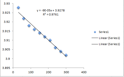
The experiment began with the analysis of Boyle’s Law. This was conducted by varying the volume of a sealed gas cylinder while monitoring the pressure change inside it. Meanwhile, the cylinder was connected to an air canister which was submerged in boiling water. This served as the heat source of the air inside the cylinder. Therefore, the total volume of the system was the cylinder and the canister combined. The results were then plotted on a volume vs. inverse pressure graph. Obtaining the equation of the line, the number of molecules within the gas chamber was computed for by equating the slope of the line to the proportionality constant NkT. Using the y-intercept of the equation, the volume of the canister was also obtained. The results of this are on Table W3.
Table W1: Diameter of the Piston
Table W2: Boyle's Law
Table W3: Boyle's Law Linear Equation
Charles’ Law was next analysed using the same setup, but this time with constant pressure and varying temperature. Cubes of ice were dropped one at a time into the boiling water. Each time, the change in temperature and volume was recorded. The results were then plotted on a volume vs. temperature graph and the resulting linear equation was obtained. Using the same method as in Boyle’s Law, the number of molecules was once again obtained, as well as the experimentally derived volume of the canister. The verifying factor to these equations was the obtained experimental volumes of the canister for each gas law analysed. As it turns out,
Table W4: Charles' Law
Table W5: Charles' Law Linear Equation
However, another factor can be attributed to the verification of the Gas Laws. Both experimental setups yielded best fits greater than 0.97 with Boyle’s Law at 0.9754 and Charles’ Law at 0.9934. This is testament to the accuracy of the predictions these laws make, thus strengthening their legitimacy.
On further thought, if a mass were placed on top of the piston during the Charles’ Law experiment, the pressure of the system would have increased. This would mean a decrease in the slope of the linear equation, but no change in its y-intercept.
It is evident in this experiment, that Gay-Lussac’s Law was overlooked. Should one find the need to verify this law as well, the same materials used would suffice. In order to do so, one would simply have to keep the volume constant by somehow keeping the piston from moving. Upon doing so, one can vary the temperature of the gas, while simultaneously recording the change in pressure of the system. Plotting the measurements on a pressure vs. temperature graph, then treating the graph with the same procedures as before, would yield the necessary information for this experimental setup. Overall, the computations for the number of molecules all yielded realistic results, the obtained canister volumes for each setup were consistent, and the R2 values for each graph were satisfactory, thus verifying the Ideal Gas Laws.
The experiment began with the analysis of Boyle’s Law. This was conducted by varying the volume of a sealed gas cylinder while monitoring the pressure change inside it. Meanwhile, the cylinder was connected to an air canister which was submerged in boiling water. This served as the heat source of the air inside the cylinder. Therefore, the total volume of the system was the cylinder and the canister combined. The results were then plotted on a volume vs. inverse pressure graph. Obtaining the equation of the line, the number of molecules within the gas chamber was computed for by equating the slope of the line to the proportionality constant NkT. Using the y-intercept of the equation, the volume of the canister was also obtained. The results of this are on Table W3.
Table W1: Diameter of the Piston
Diameter of Piston (m)
|
0.0325
|
Table W2: Boyle's Law
Height
(m)
|
P
(Pa)
|
V
(m3)
|
1/P
|
0.098
|
114300
|
8.12987E-05
|
8.74891E-06
|
0.097
|
114720
|
8.04691E-05
|
8.71688E-06
|
0.095
|
115200
|
7.881E-05
|
8.68056E-06
|
0.092
|
115670
|
7.63212E-05
|
8.64528E-06
|
0.089
|
116200
|
7.38325E-05
|
8.60585E-06
|
Temperature (K)
|
368.15
|
||
Table W3: Boyle's Law Linear Equation
0.0182 | |
.000007
| |
R2 Value
| |
N
|
3.58x10¹⁸
|
Volume of Chamber
|
Charles’ Law was next analysed using the same setup, but this time with constant pressure and varying temperature. Cubes of ice were dropped one at a time into the boiling water. Each time, the change in temperature and volume was recorded. The results were then plotted on a volume vs. temperature graph and the resulting linear equation was obtained. Using the same method as in Boyle’s Law, the number of molecules was once again obtained, as well as the experimentally derived volume of the canister. The verifying factor to these equations was the obtained experimental volumes of the canister for each gas law analysed. As it turns out,
Table W4: Charles' Law
Height
(m)
|
V
(m3)
|
|
0.098
|
364.15
|
8.12987E-05
|
0.083
|
355.15
|
6.8855E-05
|
0.077
|
350.15
|
6.38776E-05
|
0.069
|
343.15
|
5.72409E-05
|
0.062
|
340.35
|
5.14339E-05
|
0.06
|
338.85
|
4.97747E-05
|
0.054
|
333.25
|
4.47973E-05
|
0.05
|
329.65
|
4.14789E-05
|
P
(Pa)
|
113900
|
|
Table W5: Charles' Law Linear Equation
Slope
|
.000001 |
y-intercept
|
0.0003
|
R2 Value
|
0.9934
|
N
|
4.95x10²²
|
Volume of Chamber
|
On further thought, if a mass were placed on top of the piston during the Charles’ Law experiment, the pressure of the system would have increased. This would mean a decrease in the slope of the linear equation, but no change in its y-intercept.
It is evident in this experiment, that Gay-Lussac’s Law was overlooked. Should one find the need to verify this law as well, the same materials used would suffice. In order to do so, one would simply have to keep the volume constant by somehow keeping the piston from moving. Upon doing so, one can vary the temperature of the gas, while simultaneously recording the change in pressure of the system. Plotting the measurements on a pressure vs. temperature graph, then treating the graph with the same procedures as before, would yield the necessary information for this experimental setup. Overall, the computations for the number of molecules all yielded realistic results, the obtained canister volumes for each setup were consistent, and the R2 values for each graph were satisfactory, thus verifying the Ideal Gas Laws.